Number of Refugees accepted by the US (2002 - 2018)

Data from: http://ireports.wrapsnet.org/Interactive-Reporting/EnumType/Report?ItemPath=/rpt_WebArrivalsReports/MX%20-%20Arrivals%20by%20Nationality%20and%20Religion

Packages and Folders

# Install these packages if you don't have theme yet
# devtools::install_github("favstats/tidytemplate")
# install.packages("pacman")

pacman::p_load(tidyverse, readxl, sjmisc)

# Creates folders
# tidytemplate::data_dir()
# tidytemplate::images_dir()

Load Data

refugee_dat <- read_excel("data/refugee_dat.xls") %>% 
  drop_na(X__1) %>% 
  rename(cntry = X__1) %>% 
  select(-Religion, -X__2, -X__3, - Total) %>% 
  filter(!(str_detect(cntry, "Total|Data"))) %>% 
  gather(year, n, -cntry) %>% 
  mutate(year = str_replace(year, "CY ", "") %>% as.numeric)

refugee_dat %>% group_by(cntry) %>% tally() %>% arrange(desc(nn)) %>% .[1:10,] %>% .$cntry -> top10

## Using `n` as weighting variable

Static

year_dat <- tibble(year = c(2005, 2009, 2013, 2017), label = c("Bush II", "Obama I", "Obama II", "Trump I"))


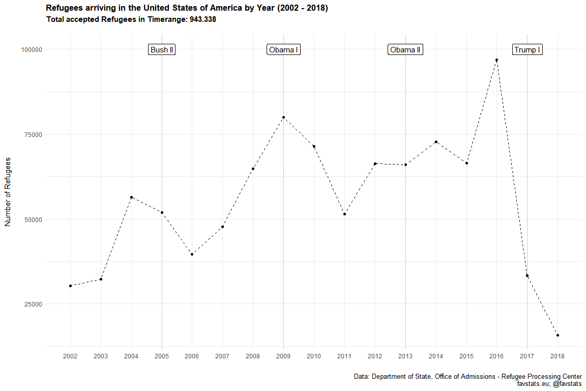
refugee_total <- refugee_dat %>% 
  group_by(year) %>% 
  tally() %>% 
  ggplot(aes(year, nn)) +
  geom_vline(data = year_dat, aes(xintercept = year), alpha = 0.15) +
  geom_label(data = year_dat, aes(x = year, y = 100000, label = label), 
            angle = 0, color = "black") +
  geom_line(linetype = "dashed") + 
  geom_point() +
  theme_minimal() +
  scale_color_manual("Country", values = qualitative) +
  theme(plot.title = element_text(size = 13, face = "bold"),
    plot.subtitle = element_text(size = 11, face = "bold"), 
    plot.caption = element_text(size = 10),
        legend.position = "bottom") +
  scale_x_continuous(breaks = 2002:2018, labels = 2002:2018) +
  labs(x = "", y = "Number of Refugees\n", 
       title = "Accepted Refugees in the United States of America by Year (2002 - 2018)", 
       subtitle = "Total accepted Refugees in Timerange: 943.338\n",
       caption = "Data: Department of State, Office of Admissions - Refugee Processing Center\n@FabioFavusMaxim; favstats.eu")

## Using `n` as weighting variable

refugee_total

tidytemplate::ggsave_it(refugee_total, width = 10, height = 6)

Colored

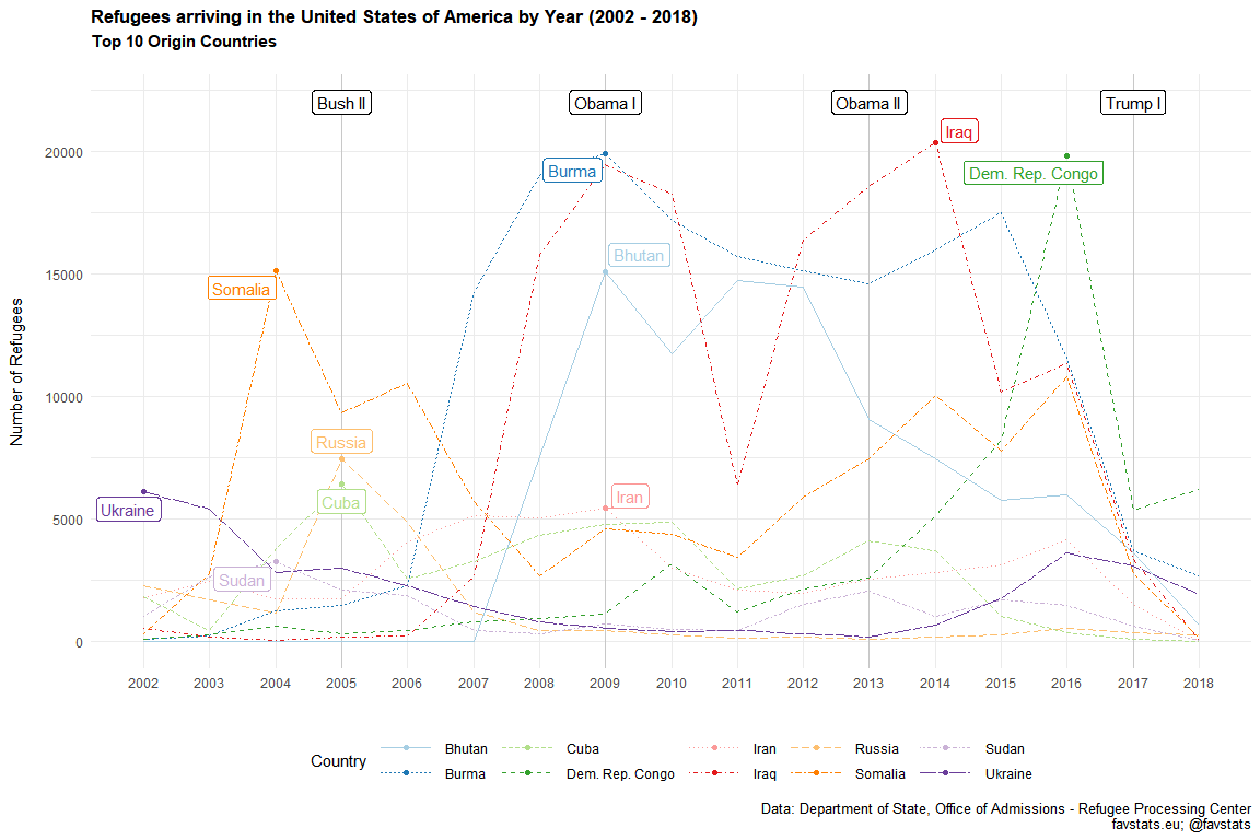
qualitative <- c('#a6cee3','#1f78b4','#b2df8a','#33a02c','#fb9a99','#e31a1c','#fdbf6f','#ff7f00','#cab2d6','#6a3d9a')

gg_refugee_static_data <- refugee_dat %>% 
  filter(cntry %in% top10) 

label_dat <- gg_refugee_static_data %>% 
  group_by(cntry) %>% 
  summarize(n = max(n)) %>% 
  select(-cntry) %>% 
  inner_join(gg_refugee_static_data)

## Joining, by = "n"

gg_refugee_static <- gg_refugee_static_data %>% 
  ggplot(aes(year, n)) +
  geom_vline(data = year_dat, aes(xintercept = year), alpha = 0.15) +
  geom_label(data = year_dat, aes(x = year, y = 22000, label = label), 
            angle = 0, color = "black") +
  geom_line(aes(linetype = cntry, color = cntry)) +
  theme_minimal() +
  ggrepel::geom_label_repel(data = label_dat, aes(label = cntry, color = cntry), show.legend = F) + 
  geom_point(data = label_dat, aes(color = cntry)) + 
  scale_color_manual("Country", values = qualitative) +
  scale_linetype("Country") +
  theme(plot.title = element_text(size = 13, face = "bold"),
    plot.subtitle = element_text(size = 11, face = "bold"), 
    plot.caption = element_text(size = 10),
    legend.key.width = unit(3, "line"),
    legend.position = "bottom") +
  scale_x_continuous(breaks = 2002:2018, labels = 2002:2018) +
  labs(x = "", y = "Number of Refugees\n", 
       title = "Accepted Refugees in the United States of America by Year (2002 - 2018)", subtitle = "Top 10 Origin Countries\n",
       caption = "Data: Department of State, Office of Admissions - Refugee Processing Center\n@FabioFavusMaxim; favstats.eu") 
  # geom_rect(aes(xmin = 2002, xmax = 2005, ymin = 22000, ymax = 22000),
  #             color = "black",
  #             alpha = 0.8,
  #             inherit.aes = FALSE)

gg_refugee_static

tidytemplate::ggsave_it(gg_refugee_static, width = 12, height = 8)

Animated

library(gganimate)

gg_refugee <- refugee_dat %>%
  filter(cntry %in% top10) %>%
  ggplot(aes(year, n, color = cntry)) +
  geom_vline(data = year_dat, aes(xintercept = year), alpha = 0.15) +
  geom_label(data = year_dat, aes(x = year, y = 22000, label = label),
            angle = 0, color = "black") +
  geom_line() +
  geom_segment(aes(xend = 2018, yend = n), alpha = 0.5) +
  geom_point() +
  geom_text(aes(x = 2019, label = cntry)) +
  theme_minimal() +
  scale_color_manual("Country", values = qualitative) +
  theme(plot.title = element_text(size = 13, face = "bold"),
    plot.subtitle = element_text(size = 12, face = "bold"),
    plot.caption = element_text(size = 10),
        legend.position = "bottom") +
  scale_x_continuous(breaks = 2002:2018, labels = 2002:2018) +
  labs(x = "", y = "Number of Refugees\n",
       title = "Accepted Refugees in the United States of America by Year (2002 - 2018)", subtitle = "Top 10 Origin Countries\n",
       caption = "Data: Department of State, Office of Admissions - Refugee Processing Center\n@FabioFavusMaxim; favstats.eu")  +
  guides(color = F, text = F) +
  transition_reveal(cntry, year, keep_last = T)

gg_refugee %>% animate(
  nframes = 500, fps = 15, width = 1000, height = 600, detail = 1
)

anim_save("images/gg_refugee.gif")

Region

Static

gg_refugee_static_region <- refugee_dat %>% 
  mutate(continent = countrycode::countrycode(cntry, "country.name", "continent")) %>% 
  mutate(region = countrycode::countrycode(cntry, "country.name", "region")) %>%
  mutate(continent = case_when(
    continent == "Asia" ~ region,
    T ~ continent
  )) %>% 
  mutate(continent = case_when(
    cntry == "Tibet" ~ "Eastern Asia",
    cntry == "Yemen (Sanaa)" ~ "Middle East",
    cntry == "Yugoslavia" ~ "Europe",
    str_detect(cntry, "Georgia|Armenia|Azerbaijan") ~ "Central Asia",
    continent == "Western Asia" ~ "Middle East",
    T ~ continent
  )) %>% 
  # group_by(continent) %>% tally
  # filter(continent == "Western Asia")
  group_by(year, continent) %>% 
  tally() 

## Warning in countrycode::countrycode(cntry, "country.name", "continent"): Some values were not matched unambiguously: Tibet, Yemen (Sanaa), Yugoslavia

## Warning in countrycode::countrycode(cntry, "country.name", "region"): Some values were not matched unambiguously: Tibet, Yemen (Sanaa), Yugoslavia

## Using `n` as weighting variable

# gg_refugee_static_region %>% filter(continent == "Southern Asia") %>% summarize_all(sum)
  
label_dat <- gg_refugee_static_region %>% 
  group_by(continent) %>% 
  summarize(nn = max(nn)) %>% 
  select(-continent) %>% 
  inner_join(gg_refugee_static_region) %>% 
  filter(!(year == 2018 & continent == "Eastern Asia")) %>% 
  filter(!(year == 2004 & continent == "Eastern Asia")) %>% 
  mutate(nn = ifelse(continent == "Southern Asia", 10385, nn)) %>% 
  mutate(year = ifelse(continent == "Southern Asia", 2015, year))

## Joining, by = "nn"

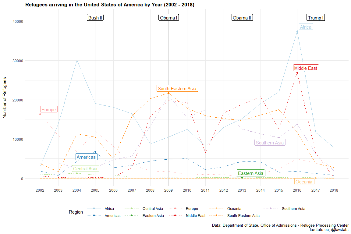
gg_static_region <- gg_refugee_static_region %>%   
  ggplot(aes(year, nn)) +
  geom_vline(data = year_dat, aes(xintercept = year), alpha = 0.15) +
  geom_label(data = year_dat, aes(x = year, y = 41000, label = label), 
            angle = 0, color = "black") +
  geom_line(aes(linetype = continent, color = continent)) +
  theme_minimal() +
  ggrepel::geom_label_repel(data = label_dat, 
                            aes(label = continent, color = continent), 
                            show.legend = F, seed = 13092018) +
  geom_point(data = label_dat, aes(color = continent)) +
  scale_color_manual("Region", values = qualitative) +
  scale_linetype("Region") +
  theme(plot.title = element_text(size = 13, face = "bold"),
    # plot.subtitle = element_text(size = 11, face = "bold"), 
    plot.caption = element_text(size = 10),
    legend.key.width = unit(3, "line"),
    legend.position = "bottom") +
  scale_x_continuous(breaks = 2002:2018, labels = 2002:2018,
                     minor_breaks = seq(2002, 2018, 1)) +
  labs(x = "", y = "Number of Refugees\n", 
       title = "Refugees arriving in the United States of America by Year (2002 - 2018)", 
       caption = "Data: Department of State, Office of Admissions - Refugee Processing Center\nfavstats.eu; @favstats") 
  # geom_rect(aes(xmin = 2002, xmax = 2005, ymin = 22000, ymax = 22000),
  #             color = "black",
  #             alpha = 0.8,
  #             inherit.aes = FALSE)

gg_static_region

tidytemplate::ggsave_it(gg_static_region, width = 12, height = 8)

Percent

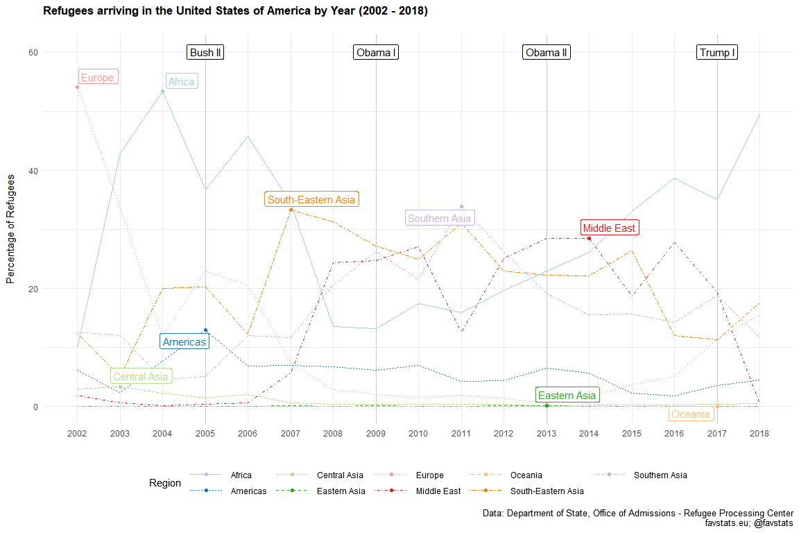
gg_static_region_perc <- gg_refugee_static_region %>% 
  group_by(year) %>% 
  mutate(total = sum(nn)) %>% 
  mutate(perc = tidytemplate::get_percentage(nn, total))  
  
label_dat <- gg_static_region_perc %>% 
  group_by(continent) %>% 
  summarize(perc = max(perc)) %>% 
  select(-continent) %>% 
  inner_join(gg_static_region_perc)

## Joining, by = "perc"

gg_region_perc <- gg_static_region_perc %>% 
  ggplot(aes(year, perc)) +
  geom_vline(data = year_dat, aes(xintercept = year), alpha = 0.15) +
  geom_label(data = year_dat, aes(x = year, y = 60, label = label),
            angle = 0, color = "black") +
  geom_line(aes(linetype = continent, color = continent)) +
  theme_minimal() +
  ggrepel::geom_label_repel(data = label_dat,
                            aes(label = continent, color = continent),
                            show.legend = F, seed = 13092018) +
  geom_point(data = label_dat, aes(color = continent)) +
  scale_color_manual("Region", values = qualitative) +
  scale_linetype("Region") +
  theme(plot.title = element_text(size = 13, face = "bold"),
    # plot.subtitle = element_text(size = 11, face = "bold"), 
    plot.caption = element_text(size = 10),
    legend.key.width = unit(3, "line"),
    legend.position = "bottom") +
  scale_x_continuous(breaks = 2002:2018, labels = 2002:2018,
                     minor_breaks = seq(2002, 2018, 1)) +
  labs(x = "", y = "Percentage of Refugees\n", 
       title = "Refugees arriving in the United States of America by Year (2002 - 2018)\n",
       caption = "Data: Department of State, Office of Admissions - Refugee Processing Center\nfavstats.eu; @favstats") 

gg_region_perc

tidytemplate::ggsave_it(gg_region_perc, width = 12, height = 8)

Animation

library(gganimate)

gg_anim_region <- gg_refugee_static_region %>%
  mutate(continent = ifelse(continent == "South-Eastern Asia", "S.E. Asia", continent)) %>% 
  ggplot(aes(year, nn, color = continent)) +
  geom_vline(data = year_dat, aes(xintercept = year), alpha = 0.15) +
  geom_label(data = year_dat, aes(x = year, y = 41000, label = label),
            angle = 0, color = "black") +
  geom_line() +
  geom_segment(aes(xend = 2018, yend = nn), alpha = 0.5) +
  geom_point() +
  geom_text(aes(x = 2019, label = continent)) +
  theme_minimal() +
  scale_color_manual("Country", values = qualitative) +
  theme(plot.title = element_text(size = 13, face = "bold"),
    # plot.subtitle = element_text(size = 12, face = "bold"),
    plot.caption = element_text(size = 10),
        legend.position = "bottom") +
  scale_x_continuous(breaks = 2002:2018, labels = 2002:2018,
                     minor_breaks = seq(2002, 2018, 1)) +
  labs(x = "", y = "Number of Refugees\n",
       title = "Refugees arriving in the United States of America by Year (2002 - 2018)\n",
       caption = "Data: Department of State, Office of Admissions - Refugee Processing Center\nfavstats.eu; @favstats")  +
  guides(color = F, text = F) +
  transition_reveal(continent, year, keep_last = T)

gg_anim_region %>% animate(
  nframes = 500, fps = 15, width = 1000, height = 600, detail = 1
)

anim_save("images/gg_anim_region.gif")

Religion Data

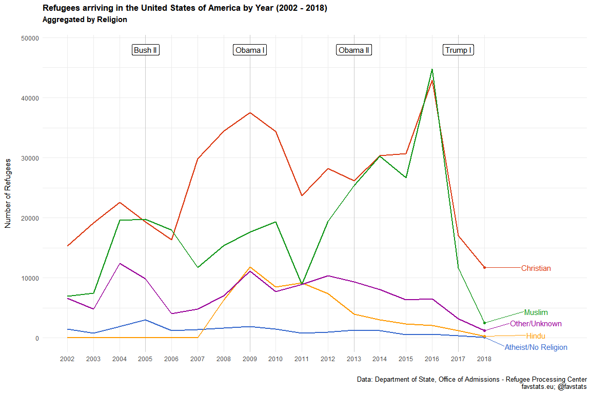
relig_refugee <- read_excel("data/refugee_dat.xls") %>% 
  drop_na(Religion) %>% 
  rename(religion = Religion) %>% 
  select(-X__1, -X__2, -X__3, - Total) %>% 
  # filter(!(str_detect(cntry, "Total|Data"))) %>% 
  gather(year, n, -religion) %>% 
  mutate(year = str_replace(year, "CY ", "") %>% as.numeric) %>% 
  # group_by(religion, year) %>% 
  # mutate(n = sum(n)) %>% 
  mutate(religion_cat = case_when(
    str_detect(religion, "Moslem|Ahmadiyya") ~ "Muslim",
    str_detect(religion, "Christ|Baptist|Chald|Coptic|Greek|Jehovah|Lutheran|Mennonite|Orthodox|Pentecostalist|Protestant|Uniate|Adventist|Cath|Meth|Old Believer") ~ "Christian",
    str_detect(religion, "Atheist|No Religion") ~ "Atheist/No Religion",
    religion == "Hindu" ~ "Hindu",
    T ~ "Other/Unknown"
  )) %>% 
  # filter(religion == "Unknown") %>% 
  # .$n %>% sum%>% 
  group_by(religion_cat, year) %>% 
  summarize(n = sum(n)) 

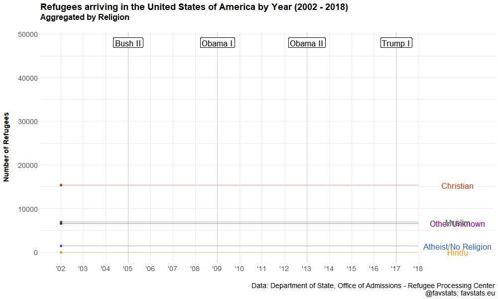
Static

label_dat <- relig_refugee %>% 
  filter(year == 2018)

gg_relig <- relig_refugee  %>% 
  ggplot(aes(year, n)) +
  geom_vline(data = year_dat, aes(xintercept = year), alpha = 0.15) +
  geom_label(data = year_dat, aes(x = year, y = 48000, label = label),
            angle = 0, color = "black") +
  geom_line(aes(color = religion_cat), size = .8) +
  theme_minimal() +
  ggrepel::geom_text_repel(data = label_dat, 
                           aes(label = religion_cat, color = religion_cat), 
                           nudge_x = 2,
                           show.legend = F, 
                           direction = "y", min.segment.length = 0.7) +
  geom_point(data = label_dat, aes(color = religion_cat)) +
  ggthemes::scale_color_gdocs("Religion") +
  # scale_color_manual("Religion", values = qualitative) +
  scale_linetype("Religion") +
  theme(plot.title = element_text(size = 13, face = "bold"),
    plot.subtitle = element_text(size = 11, face = "bold"), 
    plot.caption = element_text(size = 10),
    legend.key.width = unit(3, "line"),
    legend.position = "bottom") +
  scale_x_continuous(breaks = 2002:2018, labels = 2002:2018, 
                     limits = c(2002, 2021),
                     minor_breaks = seq(2002, 2018, 1)) +
  labs(x = "", y = "Number of Refugees\n", 
       title = "Refugees arriving in the United States of America by Year (2002 - 2018)", subtitle = "Aggregated by Religion\n",
       caption = "Data: Department of State, Office of Admissions - Refugee Processing Center\nfavstats.eu; @favstats") +
  guides(color = F)

gg_relig

tidytemplate::ggsave_it(gg_relig, width = 10, height = 6)

Animated

library(gganimate)

gg_religion <- relig_refugee %>%
  ggplot(aes(year, n, color = religion_cat)) +
  geom_vline(data = year_dat, aes(xintercept = year), alpha = 0.15) +
  geom_label(data = year_dat, aes(x = year, y = 48000, label = label),
            angle = 0, color = "black", size = 6) +
  geom_line(size = 1) +
  geom_segment(aes(xend = 2018, yend = n), alpha = 0.5) +
  geom_point(size = 2) +
  geom_text(aes(x = 2019, label = religion_cat), 
            size = 6, face = "bold", nudge_x = .75) +
  theme_minimal() +
  ggthemes::scale_color_gdocs("Religion") +
  theme(plot.title = element_text(size = 18, face = "bold"),
    plot.subtitle = element_text(size = 16, face = "bold"),
    plot.caption = element_text(size = 14),
    axis.title = element_text(size = 14, face = "bold"),
    axis.text = element_text(size = 14),
        legend.position = "bottom") +
  scale_x_continuous(breaks = 2002:2018, 
                     labels = c("'02", "'03", "'04",
                                "'05", "'06", "'07",
                                "'08", "'09", "'10",
                                "'11", "'12", "'13",
                                "'14", "'15", "'16",
                                "'17", "'18"), 
                     limits = c(2002, 2020.5),
                     minor_breaks = seq(2002, 2018, 1)) +
  labs(x = "", y = "Number of Refugees\n\n",
       title = "Refugees arriving in the United States of America by Year (2002 - 2018)", subtitle = "Aggregated by Religion\n\n",
       caption = "Data: Department of State, Office of Admissions - Refugee Processing Center\nfavstats.eu; @favstats")  +
  guides(color = F, text = F) +
  transition_reveal(religion_cat, year, keep_last = T)

gg_religion %>% animate(
  nframes = 500, fps = 15, width = 1000, height = 600, detail = 1
)

anim_save("images/gg_religion.gif")

Maps

load("data/world_map.Rdata")

refugee_map_total <- refugee_dat %>% 
  mutate(id = countrycode::countrycode(cntry, "country.name", "country.name")) %>% 
  mutate(id = ifelse(cntry == "Tibet", yes = "China", no = id)) %>%
  group_by(id) %>% 
  summarize(n = sum(n, na.rm = T)) %>% 
  full_join(world_map) %>% 
  mutate(n = cut(n,  
                 breaks = c(1, 100, 10000, 50000, 100000, 175000), 
                 labels = c("< 100", "100 - 10.000", 
                          "10.001 - 50.000", "50.001 - 100.000", 
                            "100.001 - 175.000")))

Total Map

refugee_map_total %>% 
  ggplot() +
  geom_map(map = world_map,
         aes(x = long, y = lat, group = group, map_id = id),
         color = "#7f7f7f", fill = "gray80", size = 0.15) +
  geom_map(data = refugee_map_total, 
           map = world_map,
        aes(map_id  = id, 
            fill = n), size = 0.01) + 
  theme_void() +
#  scale_fill_gradient(low = "red", high = "blue") + 
  coord_equal() +
  viridis::scale_fill_viridis("Number of Refugees", 
                              direction = -1,
                              option = "D", 
                              discrete = T, 
                              # begin = .2, 
                              # end = .8, 
                              na.value = "grey",
                        #       limits = c(0, 1), 
                        # breaks = c(0, .20, .40, .60, .8, 1),
                        labels = c("< 100", "100 - 10.000", 
                          "10.000 - 50.000", "50.000 - 100.000", 
                            "100.000 - 175.000", "No Refugees")) +
  # facet_wrap(~year, ncol = 6) +
  theme(
    plot.title = element_text(size = 18, face = "bold", hjust = 0.5),
    plot.caption = element_text(size = 14),
    legend.justification = c(1, 0),
    legend.position = c(0.2, 0.25),
    legend.title = element_text(size = 10), 
    #axis.ticks.length = unit(3, "cm"),
    legend.direction = "vertical") +
  # guides(fill = guide_colorbar(barwidth = 0.7, barheight = 15,
  #               title.position = "bottom", title.hjust = 0.5,
  #               label.theme = element_text(colour = "black", size = 6, angle = 0))) +
  labs(x = "", y = "",
       title = "Refugees arriving in the United States of America by Nationality (2002 - 2018)",
       caption = "Data: Department of State, Office of Admissions - Refugee Processing Center   \nfavstats.eu; @favstats   ")   

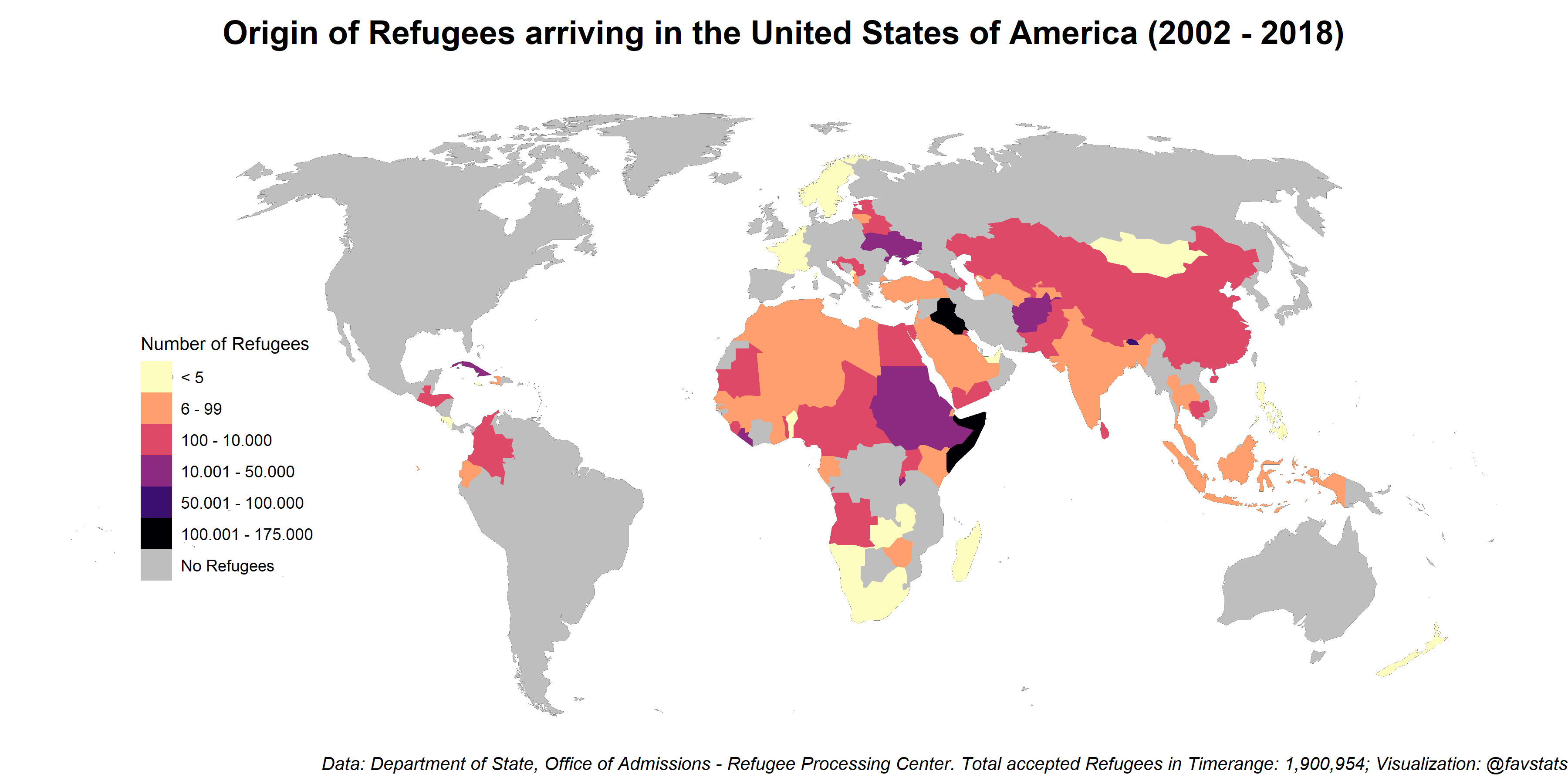
ggsave(filename = "images/refugee_total_map.png", height = 6, width = 12) 

Extended Data (1975 - 2018)

refuge_admissions75 <- 'https://static1.squarespace.com/static/580e4274e58c624696efadc6/t/5b8ff632aa4a999f85f99e8d/1536161330411/Graph+Refugee+Admissions+since+1975%289.5.18%29.pdf'

# Extract the table
out <- extract_tables(refuge_admissions75)

first_pages <- do.call(rbind, out[-length(out)]) %>% as_tibble()

correct_names <- first_pages[2,] %>% as.character()

final1 <- first_pages %>% 
  set_names(correct_names) %>% 
  .[-c(1:2),] %>% 
  .[-c(length(.)),] 

last_page <- cbind(
   out[[3]][,1],
   out[[3]][,2],
   out[[3]][,3],
   out[[3]][,5],
   out[[3]][,6],
   out[[3]][,7],
   out[[3]][,8],
   out[[3]][,9],
   out[[3]][,10],
   out[[3]][,11]
) %>% as_tibble() 
  
correct_lastpage <- last_page[2,] %>% as.character()

final2 <- last_page %>% 
  set_names(correct_lastpage) %>% 
  .[-c(1:2),] 



admissions75 <- bind_rows(final1, final2) %>% 
  select(-Total) %>% 
  mutate_all(parse_number) %>% 
  na.omit() %>% 
  gather(region, n, -`Fiscal\rYear`) %>% 
  janitor::clean_names()

Plot It

year_lab <- paste0("'", stringi::stri_sub(1975:2018, -2 , -1))

year_dat <- tibble(fiscal_year = c(seq(1976, 2016, 4)), 
                   label = c("Carter I", "Reagan I", "Reagan II", 
                             "H.W. Bush I", "Clinton I", "Clinton II", "Bush I", 
                             "Bush II", "Obama I", "Obama II", "Trump I"))

n_refugee_2018 <- admissions75 %>% 
  filter(fiscal_year == 2018) %>% 
  summarize(n = sum(n)) %>% 
  .$n

n_refugee_2002 <- admissions75 %>% 
  filter(fiscal_year == 2002) %>% 
  summarize(n = sum(n)) %>% 
  .$n

n_refugee_1992 <- admissions75 %>% 
  filter(fiscal_year == 1992) %>% 
  summarize(n = sum(n)) %>% 
  .$n

n_refugee_1980 <- admissions75 %>% 
  filter(fiscal_year == 1980) %>% 
  summarize(n = sum(n)) %>% 
  .$n

n_refugee_1975 <- admissions75 %>% 
  filter(fiscal_year == 1975) %>% 
  summarize(n = sum(n)) %>% 
  .$n

admissions75 %>% 
  summarize(n = sum(n)) %>% 
  .$n


admissions75 %>% 
  mutate(region = case_when(
    region == "Former\rSoviet\rUnion" ~ "(Former) Soviet Union",
    region == "Latin America\rCaribbean" ~ "Latin America/Caribbean",
    region == "Near East\rSouth Asia" ~ "Near East/South Asia",    
    region == "PSI" ~ "Private Sector Initiative",   
    T ~ region
  )) %>% 
  ggplot(aes(fiscal_year, n))  +
  geom_vline(data = year_dat, aes(xintercept = fiscal_year), alpha = 0.35) +
  geom_label(data = year_dat, aes(x = fiscal_year, y = 220000, label = label),
            angle = 0, color = "black") +
  geom_area(aes(fill = region), alpha = 0.9) +
  geom_hline(yintercept = n_refugee_2018, 
             linetype = "dashed", color = "black", alpha = 0.85) +
  annotate("label", x = 1978, y = 115000, 
           fill = "lightgrey", alpha = 0.85, label.size = NA,
           label = "End of\n Vietnam War") +
  annotate("label", x = 1984, y = 185000, 
           fill = "lightgrey", alpha = 0.85, label.size = NA,
           label = "Refugee Act of 1980") +
  annotate("label", x = 1997, y = 150000, 
           fill = "lightgrey", alpha = 0.85, label.size = NA,
           label = "Fall of Soviet Union") +
  annotate("label", x = 2000, y = 105000, 
           fill = "lightgrey", alpha = 0.85, label.size = NA,
           label = "Drop after 9/11") +
  annotate("label", x = 2015, y = 110000, 
           fill = "lightgrey", alpha = 0.85, label.size = NA,
           label = "Number of Refugees in 2018\n lowest since 1977") +
  theme_minimal() +
  scale_y_continuous(labels = scales::comma) +
  scale_fill_manual("Region", values = qualitative) +
  geom_curve(aes(x = 1977, y = 125000, xend = 1975, yend = n_refugee_1975),
  arrow = arrow(length = unit(0.03, "npc")), curvature = 0.2) +
  geom_curve(aes(x = 1982, y = 190000, xend = 1980, yend = n_refugee_1980),
  arrow = arrow(length = unit(0.03, "npc")), curvature = 0.2) +
  geom_curve(aes(x = 1994, y = 150000, xend = 1992, yend = n_refugee_1992),
  arrow = arrow(length = unit(0.03, "npc")), curvature = 0.2) +
  geom_curve(aes(x = 2000, y = 100000, xend = 2002, yend = n_refugee_2002),
  arrow = arrow(length = unit(0.03, "npc")), curvature = -0.3) +
  geom_curve(aes(x = 2016, y = 100000, xend = 2018, yend = n_refugee_2018),
  arrow = arrow(length = unit(0.03, "npc")), curvature = -0.2) +
  theme(plot.title = element_text(size = 13, face = "bold"),
    # plot.subtitle = element_text(size = 11, face = "bold"), 
    plot.caption = element_text(size = 10),
    legend.key.width = unit(3, "line"),
    legend.position = "bottom") +
  scale_x_continuous(breaks = 1975:2018, labels = year_lab,
                     minor_breaks = seq(1975, 2018, 1)) +
  labs(x = "", y = "Number of Refugees\n", 
       title = "Refugees arriving in the United States of America by Year (1975 - 2018)\n", 
       caption = "Data: Department of State, Office of Admissions - Refugee Processing Center\nTotal Number of Accepted Refugees since 1975: 3.340.709\nfavstats.eu; @favstats") 

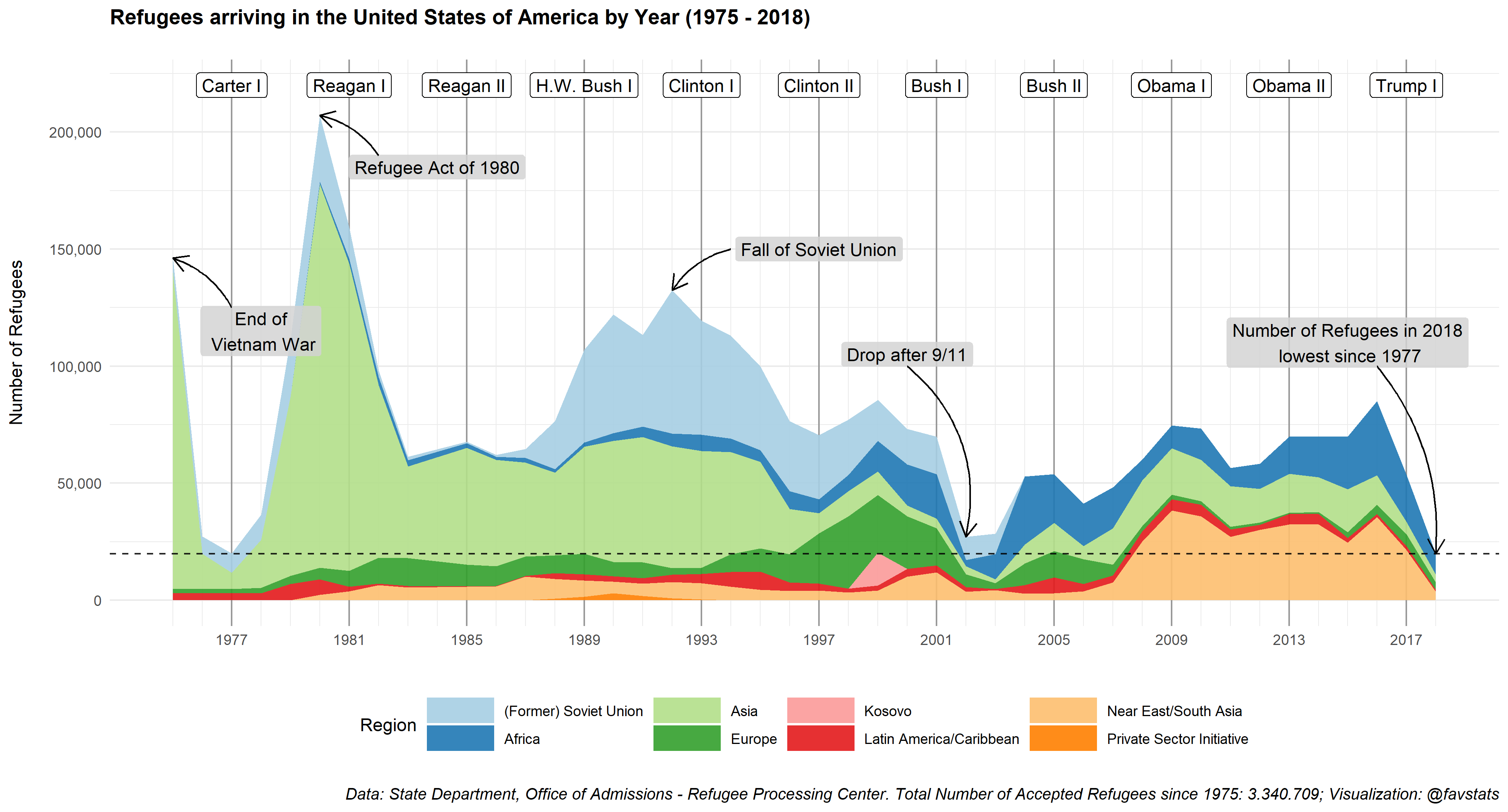
ggsave(filename = "images/refugee75.png", height = 7, width = 13)