This is a short simulation study trying to figure out the impact of collinearity on linear regressions.
Overview:
Packages
Load the necessary packages
# install pacman once if not avaible on your machine
# install.packages("pacman")

pacman::p_load(arm, purrr, MASS, broom, ggthemes, tidyverse, ecodist, viridis, gridExtra, grid, lm.beta, tidyr, ggrepel)
Simulation Function
First, I write a little function to simulate collinearity.
generate_multi <- function(n, cor_seq){
  set.seed(2017)
  x <- runif(n, 1, 10)
  models <- list()
  std.models <- list()
  for (jj in seq_along(cor_seq)) {
    ## generate correlated variable x2
    dat <- data.frame(corgen(x = x, r = cor_seq[jj],  epsilon = 0))
    colnames(dat) <- c("x1", "x2")
    ## generate y variable
    dat$y <- 0.5 * dat$x1 + 0.5 * dat$x2 + rnorm(n, sd = 10)
    ## modelling and tidy dataframe
    models[[jj]] <- tidy(lm(y ~ x1 + x2, data = dat))
    ## get standardized betas
    std.models[[jj]] <- data.frame(lm.beta::coef.lm.beta((lm.beta::lm.beta(lm(y ~ x1 + x2, data = dat)))))
    colnames(std.models[[jj]]) <- c("std.estimate")
    ## bind it together
    models[[jj]] <- std.models[[jj]] %>%
                      bind_cols(models[[jj]])
    models[[jj]]$cors <- cor_seq[jj]
  }
  sim_dat <- bind_rows(models)
  sim_dat$col <- n
  return(sim_dat)
}

draw.data <- function(cor_seq = NULL, step_seq = NULL){
    sim.list <- list()
    for(jj in seq_along(step_seq)) {
      sim.list[[jj]] <- generate_multi(n = step_seq[jj], cor_seq)
      sim.list[[jj]]$n <- step_seq[jj]

      cat(paste0("Batch: ", jj, "\t"))

    }
    sim_data <- bind_rows(sim.list)
    return(sim_data)
}
Simulate and Save Data
Draw data from function and save it.
sim_data <- draw.data(cor_seq = seq(0,.99,0.01), step_seq = seq(50, 10000, by = 50))

if(!dir.exists("data")) dir.create("data")

save(sim_data, file = "data/sim_data.Rdata")
Visualizing the Influence of Collinearity
load("data/sim_data.Rdata")
Now, consider the following linear regression: y ~ x1 + x2.
\begin{equation} Y = \beta_0 + \beta_1 X_1 + \beta_2 X_2 + \epsilon \end{equation}
For this simulation, I consistently increase the correlation between x1 and x2 (from 0 to .99) and the sample size (from 50 to 10.000) and estimate separate models for each of these combinations,
Standard Errors
First, I take a look at the impact that sample size and collinearity have on the standard error of x1. On the x-axis, you can see the increasing collinearity between x1 and x2 and the individual lines are colored in by sample size. There are a few things we can observe here: the standard error diminishes with greater sample size, correlations around .75 increase the standard error quite drastically and this effect is weaker the higher your sample size is.
get_smooths <- function(smooth_dat, n_val, y) {
  smooth_dat <- filter(smooth_dat, n == n_val & term == "x1")
  fm <- paste0(y," ~ cors")
  smooth_vals <- predict(loess(fm, smooth_dat), smooth_dat$cors)

  smooth_dat %>%
  mutate(smooth = smooth_vals) %>%
  group_by(n) %>%
  summarise(max_smooth = max(smooth),
            min_smooth = min(smooth)
            )
}

smooth_dat <- c(50, 100, 150, 200, 10000) %>%
  map_df(~get_smooths(sim_data, n_val = .x, y = "std.error")) %>%
  mutate(n_lab = ifelse(n == 50, "Sample Size: 50", n))

sim_data %>%
  filter(term == "x1") %>%
  ggplot(aes(cors, std.error, colour = n, group = n)) +
  geom_smooth(method = "loess", se = F, size = 1, alpha = 0.5) +
  xlab(expression("Pearson's"~r~correlation~between~x[1]~and~x[2])) +
  ylab(expression(x[1]~Standard~Error)) +
  theme_hc() +
  scale_color_viridis("Sample Size", direction = -1,
       breaks = seq(1000, 10000, 3000),
       labels = seq(1000, 10000, 3000)) +
  ggtitle("Sample Size and Collinearity Influence on Standard Error") +
  geom_point(data = smooth_dat, aes(x = .99, y = max_smooth)) +
  geom_text_repel(data = smooth_dat, aes(x = .99, y = max_smooth, label = n_lab),
                  nudge_y = 0.07, nudge_x = 0.03) +
  guides(colour = guide_colourbar(barwidth = 20, label.position = "bottom"))

ggsave(filename = "images/std_static.png", width = 10, height = 7)
T-Statistic and P-Values
Next, let’s take a look at the t-statistic and p-values. In line with what you would expect with greater standard errors, statistical significance also suffers from collinearity. Again, greater sample sizes seem to partly remedy this but the shift is clearly observable.
sim_data  %>%
     filter(term == "x1") %>%
     ggplot(aes(cors, statistic, colour = n, group = n)) +
     geom_smooth(method = "loess", se = F, size = 1, alpha = 0.5) +
  xlab(expression("Pearson's"~r~correlation~between~x[1]~and~x[2])) +
  ylab(expression(x[1]~t-Statistic)) +
  theme_hc() +
  scale_color_viridis("Sample Size", direction = -1,
       breaks = seq(1000, 10000, 3000),
       labels = seq(1000, 10000, 3000)) +
  geom_hline(yintercept = 1.96, linetype = "dashed", alpha = 0.9) +
  annotate(geom = "text", x = 0, y = 2.3, label = "t = 1.96") +
  ggtitle("Sample Size and Collinearity Influence on t-Statistic") +
  guides(colour = guide_colourbar(barwidth = 20, label.position = "bottom"))

ggsave(filename = "images/t_static.png", width = 10, height = 7)
sim_data  %>%
     filter(term=="x1") %>%
     ggplot(aes(cors, p.value, colour = n, group = n)) +
     geom_smooth(method = "loess", se = F, size = 1, alpha = 0.5) +
  xlab(expression("Pearson's"~r~correlation~between~x[1]~and~x[2])) +
  ylab(expression(x[1]~p-value)) +
  theme_hc() +
  scale_color_viridis("Sample Size", direction = -1,
       breaks = seq(1000, 10000, 3000),
       labels = seq(1000, 10000, 3000)) +
  geom_hline(yintercept = 0.05, linetype = "dashed", alpha = 0.9) +
  annotate(geom = "text", x = 0, y = 0.08, label = "p = 0.05") +
  ggtitle("Sample Size and Collinearity Influence on p-values") +
  guides(colour = guide_colourbar(barwidth = 20, label.position = "bottom"))

ggsave(filename = "images/p_static.png", width = 10, height = 7)
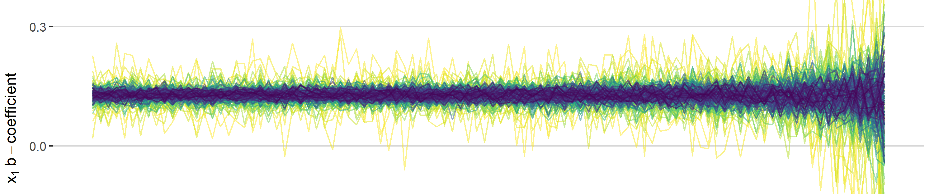
B-Coefficients
This one I find most interesting. In addition to statistical signif. being affected, you can also see how the coefficients change with increasing collinearity. The most drastic impact is for small sample sizes (~1000) where a coefficient of .5 can even become negative.
sim_data  %>%
    filter(term=="x1") %>%
    filter(n>200) %>%
    ggplot(aes(cors, estimate, colour = n, group = n)) +
    geom_hline(yintercept = 0.5, linetype = "dashed", alpha = 0.9) +
    geom_line(alpha = 0.5) +
  xlab(expression("Pearson's"~r~correlation~between~x[1]~and~x[2])) +
  ylab(expression(x[1]~b-coefficient)) +
  theme_hc() +
  scale_color_viridis("Sample Size", direction = -1,
       breaks = seq(1000, 10000, 3000),
       labels = seq(1000, 10000, 3000)) +
  annotate(geom = "text", x = 0, y = 0.08, label = "b = 0.5") +
  ggtitle("Sample Size and Collinearity Influence on b-coefficients") +
  guides(colour = guide_colourbar(barwidth = 20, label.position = "bottom"))

Animation
library(gganimate)

sim_data_sub <- sim_data  %>%
    filter(term == "x1") %>%
    filter(n > 200) %>%
    filter(n %in% c(300, 1000, 10000)) %>%
  mutate(estimate_lab = round(estimate, 2) %>% as.character) %>%
  mutate(n = as.factor(n))


 anim1 <-  sim_data_sub  %>%
    # filter(term == "x1") %>%
    # filter(n > 200) %>%
    ggplot(aes(cors, estimate, colour = n, group = n)) +
    geom_hline(yintercept = 0.5, linetype = "dashed", alpha = 0.9) +
  geom_line() +
  geom_segment(aes(xend = 1, yend = estimate), linetype = 2, colour = 'grey') +
  geom_point(size = 2) +
  geom_text(aes(x = 1, label = n), hjust = 0, size = 4, fontface = "bold") +
  geom_text(aes(x = 0.15, y = 1.8, label = paste0("Correlation: ", cors)),
                hjust = 1, size = 5, color = "black") +
  geom_text(aes(label = estimate_lab), hjust = 0, size = 3, fontface = "bold", nudge_y = 0.1) +
  xlab("Pearson's r correlation between x1 and x2") +
  ylab("x1 b-coefficient") +
  coord_cartesian(clip = 'off') +
  theme_hc() +
  scale_color_viridis("Sample Size",
                      direction = -1,
                      discrete = T,
                      begin = 0.3,
       # limits = seq(1000, 10000, 3000),
       breaks = seq(1000, 10000, 3000),
       labels = seq(1000, 10000, 3000)) +
  guides(colour = F) +
  theme(title = element_text(size = 15, face = "bold"),
        axis.text.x = element_text(size = 14, face = "bold"),
        axis.text.y = element_text(size = 10, face = "italic")) +
  ggtitle("Sample Size and Collinearity Influence on b-coefficients (Sample Sizes: 300, 1000 and 10.000)") +
  # guides(colour = guide_colourbar(barwidth = 20, label.position = "bottom")) +
  # Here comes the gganimate code
  transition_reveal(n, cors)


anim1 %>% animate(
  nframes = 500, fps = 15, width = 1000, height = 600, detail = 3
)

anim_save("images/b_anim.gif")

ggsave(filename = "images/b_static.png", width = 10, height = 7)
Standardized
Same spiel, just this time with standardized coefficients.
sim_data  %>%
     filter(term=="x1") %>%
     filter(n>200) %>%
     ggplot(aes(cors, std.estimate, colour = n, group = n)) +
    geom_line(alpha = 0.5) +
  xlab(expression("Pearson's"~r~correlation~between~x[1]~and~x[2])) +
  ylab(expression(x[1]~b-coefficient)) +
  theme_hc() +
  scale_color_viridis("Sample Size", direction = -1,
       breaks = seq(1000, 10000, 3000),
       labels = seq(1000, 10000, 3000)) +
  ggtitle("Sample Size and Collinearity Influence on standardized b-coefficients") +
  guides(colour = guide_colourbar(barwidth = 20, label.position = "bottom"))

ggsave(filename = "images/b_standardized_static.png", width = 10, height = 7)
Session Info
sessionInfo()
## R version 3.5.0 (2018-04-23)
## Platform: x86_64-w64-mingw32/x64 (64-bit)
## Running under: Windows 10 x64 (build 17134)
##
## Matrix products: default
##
## locale:
## [1] LC_COLLATE=German_Germany.1252  LC_CTYPE=German_Germany.1252
## [3] LC_MONETARY=German_Germany.1252 LC_NUMERIC=C
## [5] LC_TIME=German_Germany.1252
##
## attached base packages:
## [1] grid      stats     graphics  grDevices utils     datasets  methods
## [8] base
##
## other attached packages:
##  [1] bindrcpp_0.2.2     ggrepel_0.8.0      lm.beta_1.5-1
##  [4] gridExtra_2.3      viridis_0.5.1      viridisLite_0.3.0
##  [7] ecodist_2.0.1      forcats_0.3.0      stringr_1.3.0
## [10] dplyr_0.7.5        readr_1.1.1        tidyr_0.8.1
## [13] tibble_1.4.2       ggplot2_3.0.0.9000 tidyverse_1.2.1
## [16] ggthemes_4.0.0     broom_0.4.4        purrr_0.2.4
## [19] arm_1.10-1         lme4_1.1-17        Matrix_1.2-14
## [22] MASS_7.3-49
##
## loaded via a namespace (and not attached):
##  [1] Rcpp_0.12.18     lubridate_1.7.4  lattice_0.20-35  assertthat_0.2.0
##  [5] rprojroot_1.3-2  digest_0.6.15    psych_1.8.3.3    R6_2.2.2
##  [9] cellranger_1.1.0 plyr_1.8.4       backports_1.1.2  evaluate_0.10.1
## [13] coda_0.19-1      httr_1.3.1       pillar_1.2.1     rlang_0.2.1
## [17] lazyeval_0.2.1   readxl_1.1.0     minqa_1.2.4      rstudioapi_0.7
## [21] nloptr_1.0.4     rmarkdown_1.9    labeling_0.3     splines_3.5.0
## [25] foreign_0.8-70   munsell_0.4.3    compiler_3.5.0   modelr_0.1.1
## [29] pkgconfig_2.0.1  mnormt_1.5-5     htmltools_0.3.6  tidyselect_0.2.4
## [33] crayon_1.3.4     withr_2.1.2      nlme_3.1-137     jsonlite_1.5
## [37] gtable_0.2.0     pacman_0.4.6     magrittr_1.5     scales_0.5.0
## [41] cli_1.0.0        stringi_1.1.7    reshape2_1.4.3   xml2_1.2.0
## [45] tools_3.5.0      glue_1.3.0       hms_0.4.2        abind_1.4-5
## [49] parallel_3.5.0   yaml_2.1.19      colorspace_1.4-0 rvest_0.3.2
## [53] knitr_1.20       bindr_0.1.1      haven_1.1.2