538 Predictions for the 2018 Midterm Elections

Packages

# Install these packages if you don't have them yet
# if (!require("pacman")) install.packages("pacman")
# devtools::install_github("favstats/tidytemplate")

pacman::p_load(tidyverse, tidytemplate, janitor, ggthemes, ggpubr, rvest, ggrepel)

Load Data

csv_link <- "https://blogs.sciencemag.org/sciencehound/wp-content/uploads/sites/5/2018/11/Congressional-election-results-and-forecasts.csv"

pred_dat <- read_csv(csv_link) %>% 
  clean_names() %>% 
  mutate(close = ifelse(election_results <= 55 & election_results >= 45, "Close", "Safe")) %>% 
  left_join(tibble(state = state.name, abbr =state.abb)) %>% 
  mutate(distr_abbr = paste0(abbr, district))

pred_dat

## # A tibble: 435 x 14
##    state district democratic_cand~ republican_cand~ election_results
##    <chr>    <int> <chr>            <chr>                       <dbl>
##  1 Alab~        1 Kennedy          Byrne                        36.7
##  2 Alab~        2 Isner            Roby                         38.5
##  3 Alab~        3 Hagan            Rogers                       36.2
##  4 Alab~        4 Auman            Aderholt                     20.1
##  5 Alab~        5 Joffrion         Brooks                       38.9
##  6 Alab~        6 Kline            Palmer                       30.7
##  7 Alab~        7 Sewell           -                           100  
##  8 Alas~        1 Glavin           Young                        46  
##  9 Ariz~        1 O'Halleran       Rogers                       53.8
## 10 Ariz~        2 Kirkpatrick      Peterson                     54.4
## # ... with 425 more rows, and 9 more variables: predicted_lite <dbl>,
## #   predicted_classic <dbl>, predicted_deluxe <dbl>,
## #   predicted_probability_deluxe <dbl>, correct_deluxe <int>,
## #   democratic_win <int>, close <chr>, abbr <chr>, distr_abbr <chr>

How did 538 Predictions fare in the 2018 Midterm Elections?

text_dat <- pred_dat %>% 
  count(correct_deluxe) %>%
  spread(correct_deluxe, n) %>% 
  rename(incorrect = `0`, correct = `1`) %>%
  mutate(total = (incorrect + correct)) %>% 
  mutate(perc_correct = round(((correct / total)*100), 2)) %>% 
  mutate(label = glue::glue("538 predicted {correct} out of {total} races correctly ({perc_correct}%)"))

pred_dat %>% 
  mutate(correct_deluxe = as.factor(correct_deluxe)) %>% 
  ggplot(aes(predicted_deluxe, election_results)) +
  geom_point(aes(color = correct_deluxe)) +
  theme_minimal() +
  scale_color_colorblind() +
  geom_smooth(method = "lm", color = "black", alpha = 0.4) +
  theme(legend.position = "bottom") +
  geom_text(data = text_dat, aes(x = 22, y = 97, label = label)) + 
  labs(title = "How did 538 Predictions fare in the 2018 Midterm Elections?",
       x="Forecast from 538 Deluxe forecast % for Democratic candidates", 
       y="Actual % for Democratic candidates from the election",
       subtitle = "Black dots show 10 races that were wrongly predicted",
       caption = "favstats.eu; @favstats\nData: @jeremymberg")  +
  guides(color = F)  +
  theme(plot.title = element_text(size = 13, face = "bold"),
    plot.subtitle = element_text(size = 11, face = "italic"))

ggsave_it(pred1, width = 10, height = 6)

How did 538 Predictions fare in the 2018 Midterm Elections? - Close Races

pred_dat %>% 
  ggplot(aes(predicted_deluxe, election_results)) +
  geom_point(aes(color = close)) +
  theme_minimal() +
  scale_color_colorblind() +
  geom_hline(yintercept = 55, linetype = "dashed") +
  geom_hline(yintercept = 45, linetype = "dashed") +
  geom_smooth(method = "lm", color = "black", alpha = 0.4) +
  theme(legend.position = "bottom") +
  stat_cor() +
  labs(title = "How did 538 Predictions fare in the 2018 Midterm Elections?",
       x="Forecast from 538 Deluxe forecast % for Democratic candidates",
       y="Actual % for Democratic candidates from the election",
       subtitle = "Black dots show 89 races that were close",
       caption = "favstats.eu; @favstats\nData: @jeremymberg")  +
  guides(color = F)  +
  theme(plot.title = element_text(size = 13, face = "bold"),
    plot.subtitle = element_text(size = 11, face = "italic"))

ggsave_it(pred2, width = 10, height = 6)

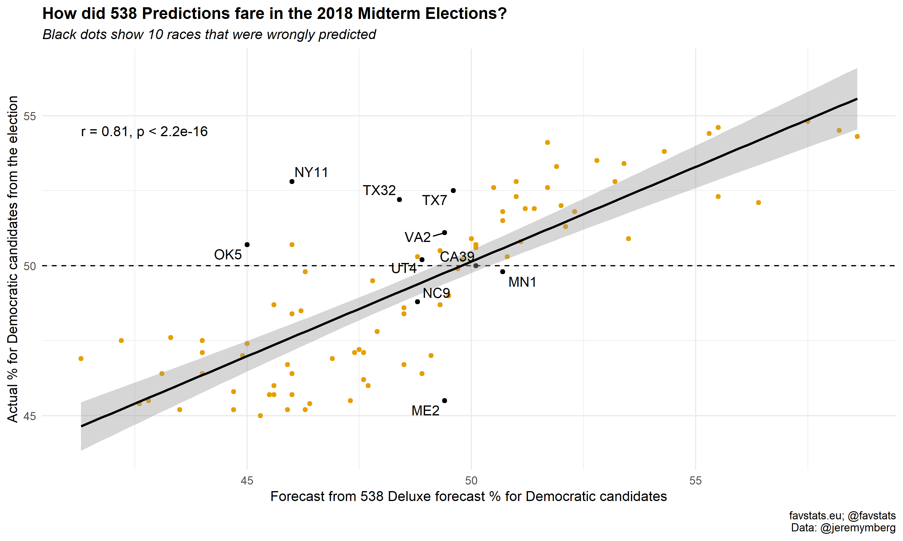
How did 538 Predictions fare in the 2018 Midterm Elections? - Close Races II

pred_dat %>% 
  mutate(correct_deluxe = as.factor(correct_deluxe)) %>% 
  filter(close == "Close") %>% 
  ggplot(aes(predicted_deluxe, election_results)) +
  geom_point(aes(color = correct_deluxe)) +
  theme_minimal() +
  geom_hline(yintercept = 50, linetype = "dashed") +
  scale_color_colorblind() +
  scale_y_continuous(breaks = c(45, 50, 55)) +
  geom_smooth(method = "lm", color = "black", alpha = 0.4) +
  geom_text_repel(data = pred_dat %>% filter(correct_deluxe == 0), aes(label = distr_abbr)) +
  theme(legend.position = "bottom") +
  stat_cor() +
  labs(title = "How did 538 Predictions fare in the 2018 Midterm Elections?",
       x="Forecast from 538 Deluxe forecast % for Democratic candidates", 
       y="Actual % for Democratic candidates from the election",
       subtitle = "Black dots show 10 races that were wrongly predicted",
       caption = "favstats.eu; @favstats\nData: @jeremymberg")  +
  guides(color = F)  +
  theme(plot.title = element_text(size = 13, face = "bold"),
    plot.subtitle = element_text(size = 11, face = "italic"))

ggsave_it(pred3, width = 10, height = 6)

How did 538 Predictions fare in the 2018 Midterm Elections? - Prediction

hist_dat <- pred_dat %>% 
  mutate(diff = abs(election_results - predicted_deluxe)) %>% 
  arrange(desc(diff)) 

difference <- mean(hist_dat$diff) %>% round(2)

hist_dat %>% 
  ggplot(aes(diff)) +
  theme_minimal() +
  geom_histogram(alpha = 0.75) +
  geom_vline(xintercept = difference, linetype = "dashed") +
  geom_text(aes(x = difference + .5, y = 62, label = difference)) +
  labs(title = "How did 538 Predictions fare in the 2018 Midterm Elections?",
       x="Absolute Difference between 538 Forecast and Results in %", 
       y="Frequency",
       caption = "favstats.eu; @favstats\nData: @jeremymberg")  +
  guides(color = F)  +
  theme(plot.title = element_text(size = 13, face = "bold"))

## `stat_bin()` using `bins = 30`. Pick better value with `binwidth`.

ggsave_it(pred4, width = 10, height = 6)